Quickstart
Tutorial prerequisites
A suitable python shell (e.g. Anaconda)
Knowledge of XML (this video can serve as a nice introduction)
Fastest-lap can be very easily invoked from scripting languages such as Python and MATLAB. Let’s do a super fast and simple system test: let’s compute a lap around Circuit de Catalunya using Python.
This example is based on the python notebook 1-simple-lap that can be found in the repository.
The entry point to fastest-lap, is the file fastest_lap.py. It is located under examples/python for Mac and Linux, and under include for Windows. This file already knows how to find the C++ dynamic library, so you do not need to worry about it.
We start by including the fastest_lap module. In this tutorial, every string called as "/path/to/whatever" is a placeholder for you to introduce the real path in your system to the indicated file.
import sys,os,inspect
sys.path.append("/path/to/folder/where/fastest_lap.py/is/found/")
import fastest_lap
This command imports the Fastest-lap python API functions, and also loads the C++ library. The C++ library is a collection of functions responsible of the computations, plus its internal memory where cars, circuits, and results are stored. From this point, Fastest-lap is ready.
We can create a car model from an XML data file by calling create_vehicle_from_xml()
vehicle_name = "car"
fastest_lap.create_vehicle_from_xml(vehicle_name, "/path/to/database/vehicles/f1/mercedes-2020-catalunya.xml");
This creates a variable of type 3dof F1 car in the Fastest-lap C++ internal memory by the name of "car". If you try to create another variable with the same name, the application will throw an error.
Next, we can load a circuit from an XML file by calling create_track_from_xml(). This XML file contains a mesh of the track centerline, and precomputed values for the heading angle, curvature, and distance to the track limits.
track_name = "catalunya"
fastest_lap.create_track_from_xml(track_name, "/path/to/database/tracks/catalunya/catalunya_adapted.xml");
This creates a variable of type track in the internal memory with the name "catalunya". We can retrieve additional data from the track that is needed for future calculations, such as the arclength (traveled distance along the track centerline) mesh. We can do so by calling track_download_data()
s = fastest_lap.track_download_data(track_name,"arclength");
Car and circuit are ready. Let’s compute the optimal laptime. We start by setting the options configure the computation. Options are passed through a string written in XML format. For now, we will just set two options:
First, the simulation produces timeseries for the dynamic variables (think of the velocity, positions, forces, etc). These are stored as variables in the Fastest-lap internal memory that can be later retrieved. We just must specify a virtual folder where these variables will be stored, in this case we use
"run/". The velocity will be later accessed asrun/chassis.velocity.x.Second, while the simulator runs we can have some screen output to see the progress. This output is redirected from Ipopt, and it has up to 12 print levels (print level 0 produces no output). We chose
print_level = 5, as it gives enough representative data of how the solution is converging.
options  = "<options>"
options += "    <output_variables>"
options += "        <prefix>run/</prefix>"
options += "    </output_variables>"
options += "    <print_level> 5 </print_level>"
options += "</options>"
Check in this link the full list of options available.
To compute the laptime, we call optimal_laptime(). We pass to this funciton the vehicle, the track, the arclength mesh, and the options.
Its output is the names of all the generated variables in the internal memory.
We can redirect this data to fastest_lap.download_variables(), which downloads the variables to the python workspace.
This variables are stored in a dictionary run and they can be accessed by name (e.g. x = run["chassis.position.x"]).
run = fastest_lap.download_variables(*fastest_lap.optimal_laptime(vehicle_name, track_name, s, options));
This is Ipopt version 3.14.8, running with linear solver MUMPS 5.5.0.

Number of nonzeros in equality constraint Jacobian...:   154734
Number of nonzeros in inequality constraint Jacobian.:    18122
Number of nonzeros in Lagrangian Hessian.............:    85034

Total number of variables............................:    10455
                    variables with only lower bounds:        0
                variables with lower and upper bounds:    10455
                    variables with only upper bounds:        0
Total number of equality constraints.................:     9061
Total number of inequality constraints...............:     4182
        inequality constraints with only lower bounds:        0
inequality constraints with lower and upper bounds:     4182
        inequality constraints with only upper bounds:        0

iter    objective    inf_pr   inf_du lg(mu)  ||d||  lg(rg) alpha_du alpha_pr  ls
0  3.3056907e+02 2.69e-01 4.57e-02  -1.0 0.00e+00    -  0.00e+00 0.00e+00   0
1  3.2889671e+02 1.14e+00 8.46e-01  -1.0 1.18e+00    -  7.05e-01 1.00e+00f  1
2  3.1958071e+02 3.11e-01 1.13e-01  -1.0 4.22e-01    -  8.49e-01 1.00e+00f  1
3  1.6821222e+02 2.80e+00 7.32e-01  -1.0 1.94e+01    -  6.60e-01 1.00e+00f  1
4  1.2837223e+02 1.21e+00 6.27e-01  -1.0 2.09e+01    -  6.77e-01 1.00e+00f  1
5  9.9468468e+01 8.94e-01 7.43e-01  -1.0 2.36e+01    -  6.96e-01 1.00e+00f  1
6  9.2840692e+01 5.66e-01 3.26e-01  -1.7 9.36e+00    -  8.21e-01 1.00e+00h  1
7  8.5271100e+01 4.41e-01 1.41e-01  -1.7 1.11e+01    -  1.00e+00 1.00e+00f  1
8  8.5277352e+01 6.13e-02 5.65e-01  -1.7 5.96e-01   0.0 1.00e+00 1.00e+00h  1
9  8.5278537e+01 1.74e-03 2.30e-01  -1.7 8.39e-02   0.4 1.00e+00 1.00e+00h  1
iter    objective    inf_pr   inf_du lg(mu)  ||d||  lg(rg) alpha_du alpha_pr  ls
10  8.5276892e+01 1.53e-04 1.03e-02  -1.7 1.16e-02  -0.1 1.00e+00 1.00e+00h  1
11  8.0956232e+01 3.37e-01 1.06e-01  -3.8 8.10e+00    -  6.33e-01 6.48e-01f  1
12  7.8792474e+01 2.86e-01 1.13e-01  -3.8 1.02e+01    -  5.74e-01 3.43e-01h  1
13  7.6337073e+01 2.45e-01 1.30e-01  -3.8 1.14e+01    -  2.85e-01 4.48e-01h  1
14  7.6345553e+01 1.69e-01 1.58e+00  -3.8 3.10e-01  -0.5 2.83e-02 1.00e+00h  1
15  7.6346316e+01 5.11e-02 9.21e-01  -3.8 1.20e-01  -0.1 8.55e-01 1.00e+00h  1
16  7.6329460e+01 9.29e-03 2.23e-01  -3.8 5.64e-02  -0.6 1.00e+00 1.00e+00h  1
17  7.6287363e+01 8.06e-03 4.78e-02  -3.8 1.29e-01  -1.1 1.00e+00 1.00e+00h  1
18  7.6185877e+01 1.64e-02 3.11e-02  -3.8 2.66e-01  -1.5 1.00e+00 1.00e+00h  1
19  7.6127662e+01 8.19e-02 4.57e-02  -3.8 9.62e-01  -2.0 3.67e-01 2.42e-01h  1
iter    objective    inf_pr   inf_du lg(mu)  ||d||  lg(rg) alpha_du alpha_pr  ls
20  7.6118606e+01 3.31e-02 1.29e-01  -3.8 2.20e-01  -0.7 1.00e+00 1.00e+00h  1
21  7.6085306e+01 1.53e-03 5.87e-03  -3.8 8.50e-02  -1.2 1.00e+00 1.00e+00h  1
22  7.5992174e+01 1.20e-02 6.35e-03  -3.8 2.57e-01  -1.6 1.00e+00 1.00e+00h  1
23  7.5866448e+01 3.66e-02 2.11e-01  -3.8 5.46e-01  -2.1 2.75e-01 5.12e-01h  1
24  7.5782968e+01 3.18e-02 3.21e-01  -3.8 1.38e+00  -2.6 1.00e+00 1.34e-01h  1
25  7.5574503e+01 2.03e-02 2.85e-01  -3.8 3.08e-01  -2.2 3.78e-01 9.34e-01h  1
26  7.5372005e+01 1.57e-02 2.10e-01  -3.8 7.58e-01  -2.6 1.00e+00 3.63e-01h  1
27  7.5209407e+01 1.00e-02 2.79e-02  -3.8 2.86e-01  -2.2 1.00e+00 8.62e-01h  1
28  7.5140991e+01 2.26e-03 1.74e-03  -3.8 1.07e-01  -1.8 1.00e+00 1.00e+00h  1
...
...
110  7.3367142e+01 1.39e-04 3.83e-04  -8.6 7.39e-01    -  9.87e-01 9.57e-01h  1
111  7.3367124e+01 8.70e-06 9.28e-07  -8.6 2.18e-01    -  1.00e+00 1.00e+00h  1
112  7.3367124e+01 1.91e-07 6.65e-08  -8.6 3.83e-02    -  1.00e+00 1.00e+00h  1
113  7.3367124e+01 4.79e-09 1.72e-09  -8.6 1.76e-03    -  1.00e+00 1.00e+00h  1
114  7.3367123e+01 4.94e-09 1.06e-09 -11.0 4.98e-03    -  1.00e+00 1.00e+00h  1
115  7.3367123e+01 5.14e-12 3.13e-13 -11.0 2.68e-05    -  1.00e+00 1.00e+00h  1

Number of Iterations....: 115

                                (scaled)                 (unscaled)
Objective...............:   7.3367123134545238e+01    7.3367123134545238e+01
Dual infeasibility......:   3.1333330545970075e-13    3.1333330545970075e-13
Constraint violation....:   5.1400678418439538e-12    5.1400678418439538e-12
Variable bound violation:   9.3933291700487587e-11    9.3933291700487587e-11
Complementarity.........:   9.9178403300925627e-12    9.9178403300925627e-12
Overall NLP error.......:   9.9178403300925627e-12    9.9178403300925627e-12


Number of objective function evaluations             = 121
Number of objective gradient evaluations             = 116
Number of equality constraint evaluations            = 121
Number of inequality constraint evaluations          = 121
Number of equality constraint Jacobian evaluations   = 116
Number of inequality constraint Jacobian evaluations = 116
Number of Lagrangian Hessian evaluations             = 115
Total seconds in IPOPT                               = 82.715

EXIT: Optimal Solution Found.
After approximately 1 minute, the results should be ready. You can plot, analyze, and visualize all the data stored in run.
You can list all the available variables calling run.keys().
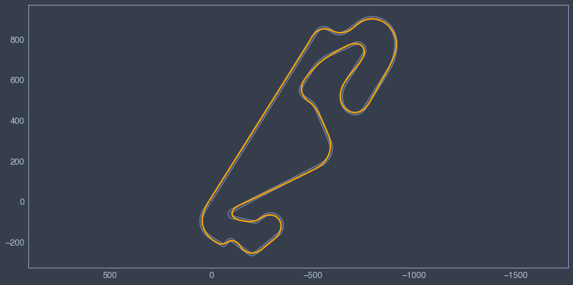
A quick way to plot the trajectory is calling plot_optimal_laptime
import numpy as np
fastest_lap.plot_optimal_laptime(s, run["chassis.position.x"], run["chassis.position.y"], track_name);
plt.gca().invert_xaxis()
And that’s all folks, I hope you enjoy it!